What is inside an OLAP cube and why we need a special data structure for it? What is the difference between OLAP cube and the data in a relational database?
When I tried to find information about the data model behind OLAP cubes. It appeared not so easy. First, there is no common approach to OLAP. Each vendor use own physical model of the cube and own algorithm. Second, the multidimensional approaches far more complex then approaches used for relational databases. This post describes one of the approaches.
Let’s consider a simplistic example: there are tree dimensions – Product, Customer and Date. The fact is a sale of a product to a customer on a date. The measures could be the number of items sold and the total price. Both in OLAP and RDB, we store this data as a list of records. Each record contains the reference to the product sold, the customer, the date, the number of items sold and the total price. The difference is aggregations and indexing.
To provide consistent performance OLAP system stores and maintains aggregations for all possible subsets of dimensions (well, not always “all”). A cube base on a subset of dimensions is called cuboid or group-by. For n-dimensional cube there are 2^n dimension combinations. So the full data cube has 1 base cube and 2^n-1 cuboids. E.g.
- Base cube: (Product, Customer, Time)
- 2 dimensional cuboids: (Product, Customer), (Customer, Time), (Product, Time)
- 1 dimensional cuboids: (Product), (Customer), (Time)
- 0 dimensional cuboid.
This inherent feature of OLAP system can be modeled in RDB but this is not so easy and natural. The indented use of OLAP is ad hoc queries, with unpredictable set of dimensions, therefore the best solution would be to store all possible combinations. RDB is mostly used for a settled number of queries, so storing many aggregations could be wasteful.
Another requirement is the consistent performance of slicing (when one or more attributes are restricted to a single value). RDB indexes are usually not good for this purpose. Multidimensional data requires multidimensional access methods. The basic problem is the nature of multidimensional data:
There exists no total ordering among spatial objects that preserves spatial proximity. In other words, there is no mapping from two- or higher- dimensional space into one-dimensional space such that any two objects that are spatially close in the higher-dimensional space are also close to each other in the one-dimensional sorted sequence. This makes the design of efficient access methods in the spatial domain much more difficult than in traditional databases, where a broad range of efficient and well-understood access methods is available.
A solution is to use heuristics that preserves spatial proximity at least to some extent. One of the efficient approaches is Hilbert R-Tree.
Hilbert R-Tree
Let’s consider 2 dimensional cuboid e.g. Product, Time.

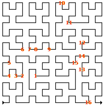
We build a Hilbert space filling curve. It will give us a basis for one dimensional ordering of the data.

One dimensional ordering is necessary as the data is stored on the disk which has one dimensional nature. It is important to store the data in an order that allows efficient multidimensional queries. In case of Hilbert space filling curve, it is possible to build an efficient index.

In one dimensional space, B-tree (balanced tree) is commonly used for indexes, it allows searches, sequential access, insertions, and deletions in logarithmic time. In multidimensional space, R-tree is often used. R-tree is generalization of B-tree. It groups nearby points and represents them with their minimum bounding rectangle in the next higher level of the tree.
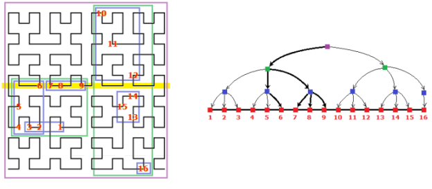
Hilbert R-tree is an R-tree variant that uses the Hilbert curve to impose a linear ordering on the data rectangles. Hilbert-Pack algorithm can be used to create the R-tree.
In the example, we group points 1..3 into first rectangle, 4..5 into second rectangle, 7..9 into third rectangle. After this, these three rectangles are covered with fourth rectangle. This fourth rectangle is the minimum bounding rectangle of the first three. And so on.
The result is a balanced tree (all leaf nodes are on the same level). The maximum number of rectangles in a node called capacity. In the example it is 3.

The intuitive reasons why our Hilbert-based methods will result in good performance is that the resulting R-tree nodes tend to be small square-like rectangles. This indicates that the nodes will likely have small area and small perimeters. Small area values result in good performance for point queries; small area and small perimeter values lead to good performance for larger queries. It was also shown experimentally that the Hilbert curve achieves the best clustering among other space filling curves.

Search is starting from the root, it descends the tree and examines all nodes that intersect the query rectangle (yellow). At the leaf level, it reports all entries that intersect the query rectangle as qualified data items.

Ok, that is basically it. This was short consideration of an OLAP cube structure. More details here:
- http://en.wikipedia.org/wiki/B-tree
- http://en.wikipedia.org/wiki/Spatial_index
- http://en.wikipedia.org/wiki/R-tree
- http://en.wikipedia.org/wiki/Hilbert_R-tree
- Volker Gaede “Multidimensional Access Methods”
- Ibrahim Kamel “Hilbert R-Tree: An Improved R-Tree Using Fractals”
- Nikos N. Karayannidis “Storage Structures, Query Processing and Implementation of On-Line Analytical Processing Systems” Ph.D. Thesis
- Ahmad Taleb “Query Optimization and Execution for Multi-Dimensional OLAP” Ph.D. Thesis